In the movie Hidden Figures, Dorothy Vaughan learned Fortran and used it for astronomical stuff. I assume Fortran only used single precision back then, so the rounding errors of single-precision real numbers did not affect tasks like rocket launching and space exploration? My impression is that these tasks require very high precision.
The Fortran wikipedia article says
IBM’s FORTRAN II appeared in 1958. The main enhancement was to support procedural programming by allowing user-written subroutines and functions which returned values with parameters passed by reference. The COMMON statement provided a way for subroutines to access common (or global) variables. Six new statements were introduced:[24]
SUBROUTINE,FUNCTION, andENDCALLandRETURNCOMMONOver the next few years, FORTRAN II would also add support for the
DOUBLE PRECISIONandCOMPLEXdata types.
and the article on Dorothy Vaughan says
Vaughan moved into the area of electronic computing in 1961, after NACA introduced the first digital (non-human) computers to the center. Vaughan became proficient in computer programming, teaching herself FORTRAN and teaching it to her coworkers to prepare them for the transition. She contributed to the space program through her work on the Scout Launch Vehicle Program.[10] A blog describing her work at NASA is on the Science Museum group website[12]
so she may have had access to double precision reals for her Fortran programming.
If you look at past hardware, the meaning of real was not the 32-bit format which is widespread today on x86-64:
-
UNIVAC 1100/1200
- single precision – 36 bits: sign bit, 8-bit characteristic, 27-bit mantissa
- double precision – 72 bits: sign bit, 11-bit characteristic, 60-bit mantissa
-
IBM 704
- single precision – sign bit, an 8-bit excess-128 exponent and a 27-bit magnitude.
The Science Musem blog post on Dorothy Vaughan mentions an IBM 360/195. The references pages for this machine also show it had an “extended execution unit” with a 28-digit fraction for floating point. You can read more details in IBM hexadecimal floating-point
To see how different the floating point representations were on past architectures, you can have a look at the r1mach and d1mach routines (Index of /port/Mach). @jacobwilliams wrote a blog about them recently titled D1MACH Re-Revisited. Concerning precision another interesting read I can suggest you is How Many Decimals of Pi Do We Really Need? by NASA/JPL Edu.
More importantly the engineers and scientists working in the space program went to great length to study the effect that modelling and rounding errors had on their predicted trajectories, and devised ways to correct them. The main invention here was the Kalman filter. You can read more about it in
- Muller, E. S., & Kachmar, P. M. (1970). The apollo rendezvous navigation filter theory, description and performance. MIT Charles Stark Draper Laboratory.
- McGee, L. A. (1985). Discovery of the Kalman filter as a practical tool for aerospace and industry (Vol. 86847). National Aeronautics and Space Administration.
On Page 10 of the McGee report studies of word-length effects done at Ames Research Center (ARC) are mentioned:
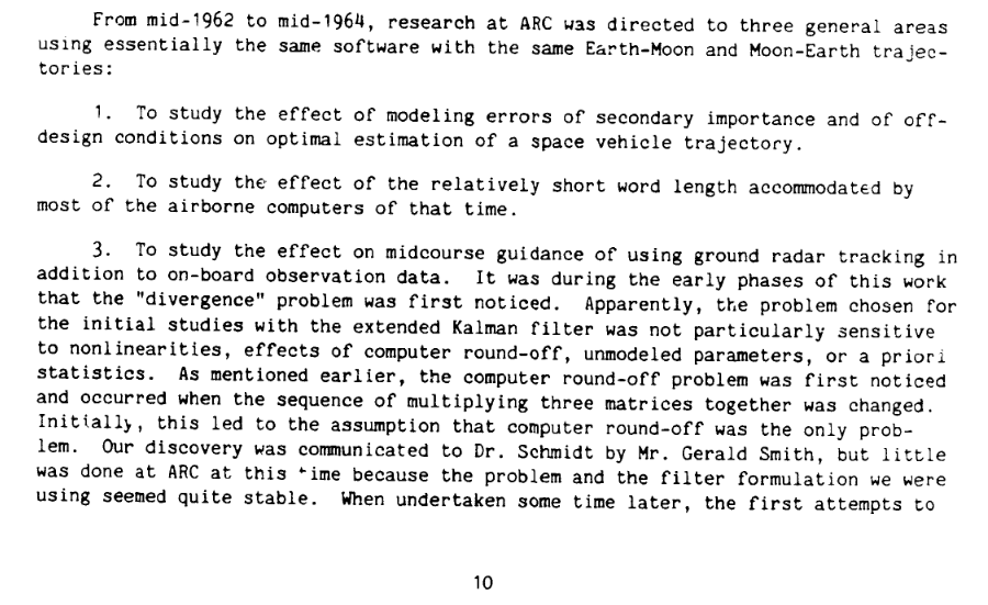
The report mentions they performed the simulations on an IBM 704.
Later in the 70’s Gerald J. Bierman from JPL did a bunch of work on stable factorization algorithms for Kalman filtering. Some of his work is described in
- Thornton, C. L., & Bierman, G. J. (1976). A numerical comparison of discrete Kalman filtering algorithms: An orbit determination case study (No. NASA-CR-148278).
- Bierman, G. J. (1977). Factorization methods for discrete sequential estimation. Academic Press, Inc., New York.
Notably, the routines Gerald Bierman and his brother Keith used in their consultancy company, Factorized Estimation Applications, Inc., were made available via Netlib:
1. a/esl.tgz
for: estimation and smoothing by UDU**T and square root information filter SRIF for Kalman filtering
by: Keith and Gerald Bierman
lang: Fortran
ref: “Factorization Methods for Discrete Sequential Estimation”, Academic Press 1977. Republished by Dover
You can read in one of the Fortran source comments:
C         Introduction
C
C The Estimation Subroutine Library (ESL) was originally authored by Gerald J.
C Bierman and Keith H. Bierman. The algorithms largely correspond closely
C to those found the Research Monograph "Factorization Methods for Discrete
C Sequential Estimation" originally published by Academic Press. It has
C been reprinted by Dover with ISBN-10: 0486449815 and ISBN-13: 978-0486449814
C
C Originally published as commerical software by Factorized Estimation
C Applications Inc. it has largely been unavailable to the general public
C for over 20 years. This library is now licensed under the Creative Commons
C Attribution 3.0 Unported License.
C To view a copy of this license, visit http://creativecommons.org/licenses/by/3.0/
C or send a letter to Creative Commons, 171 Second Street, Suite 300,
C San Francisco, California, 94105, USA.
C
C As most are aware, Gerald J. Bierman (Ph.D., IEEE Fellow) died suddenly in
C his prime in 1987. This library is re-released in his memory.
C
C Keith H. Bierman 2008
C khbkhb@gmail.com
C Cherry Hills Village, CO
For those interested, I’ve been able to locate the in memoriam for Gerald Jack Bierman. I would also bring to your attention his involvement in the Voyager orbit determination at Jupiter (1983). As he wrote there:
Numerous tests were made throughout the mission to
test estimate consistency and accuracy of the SRIF/SRIS
and U-D algorithm implementations. The navigation
estimation software performed flawlessly. Indeed, the
estimation software performed so well that most of the
time it was taken for granted by the navigation team, and
that is the ultimate compliment.
I would note that Voyager 1 & Voyager 2 remain in contact with Earth. Maybe Bierman’s Fortran factorizations are still doing their job on some NASA computer just like they did 50 years ago?
Note also that the Newtonian constant of gravitation is one of the constant known with the lowest precision (https://physics.nist.gov/cuu/Constants/):
- The 2018 value is G = 6.674 30(15) \times 10^{-11} m^3 kg^{-1} s^{-2} (=> standard uncertainty 0.000 15 \times 10^{-11} m^3 kg^{-1} s^{-2})
- The 1969 value was G = 6.673 2 (31) \times 10^{-11} m^3 kg^{-1} s^{-2}
In certain situations, like the third Kepler’s law, you can eliminate it: a^2/T^3 = const
but in the general case probably not. So I would be curious to know how computations are made in this domain to achieve so precise trajectories (New Horizons visiting Pluto then Arrokoth for example)…
To somewhat answer the original question: results itself usually do not require high precision, but some algorithms do, in particular if dealing with large complex models or lots of iterations (evolution equations). But those might not have been feasible back then.
Just one simple example, modern Krylov space methods often suffer from internal rounding errors and convergence degrades or breaks down. Double precision helps a lot (use single precision for the matrix to reduce memory bandwidth and double precision for vectors and internal operations).
Spacecraft trajectories are not calculated with G but with G*M where M is the mass of the body that the
spacecraft is orbiting. It is known to much higher accuracy than either G or M.