Fortran code snippets

[Beliavsky]

A correlation matrix of dimension n where all the off-diagonal elements have value r has an inverse matrix whose diagonal elements equal

(1 + (n-2)*r) / ((1-r) * (1 + (n-1)*r))

and off-diagonal elements equal

r / ((r-1) * (1 + (n-1)*r))

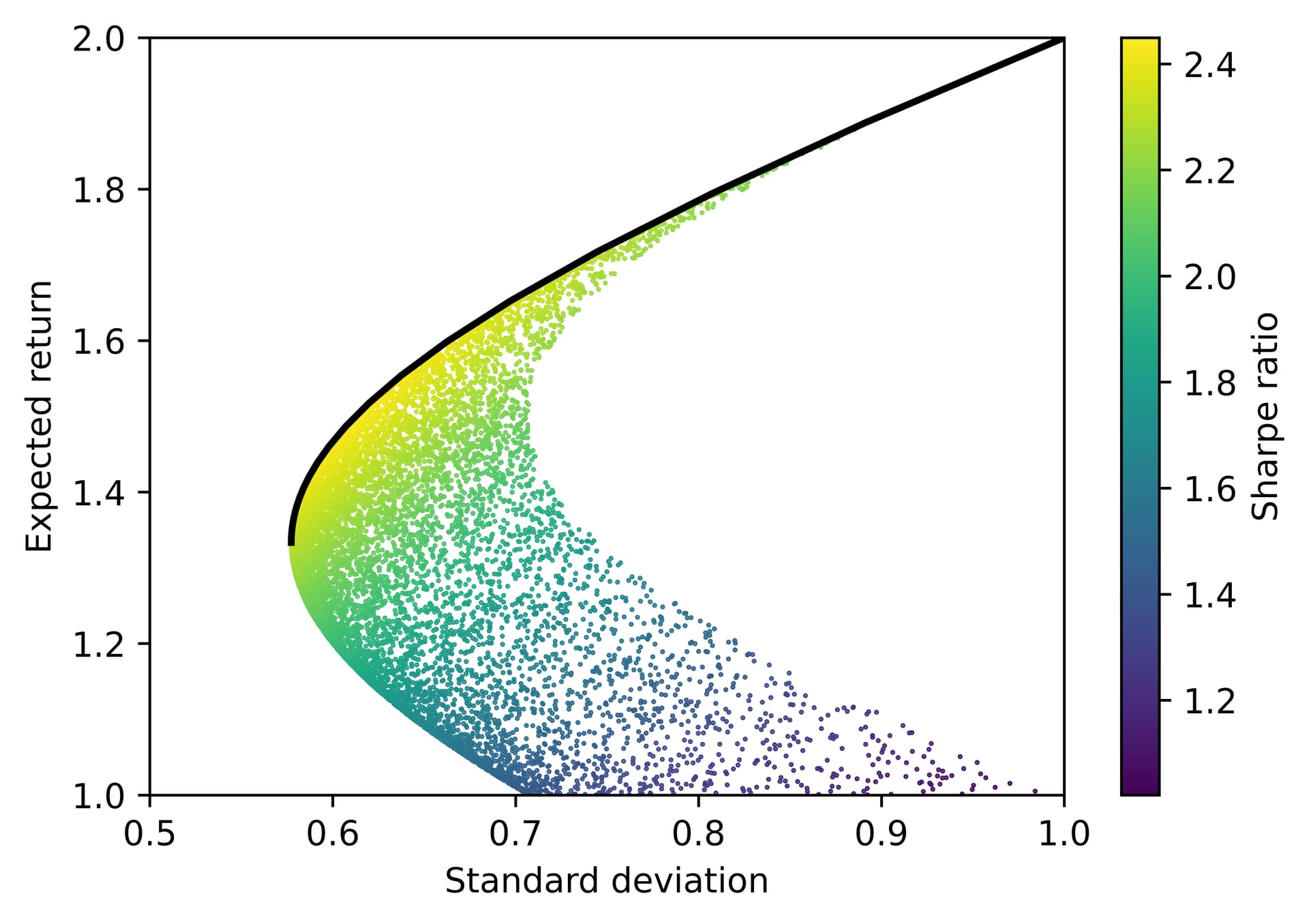
Given the expected returns mu and covariances cov of assets, when taking positions w the expected portfolio return is mu' * w, the variance is w' * cov * w, and optimal portfolio weights are proportional to cov^(-1) * mu. The program below specifies expected returns for 3 assets and studies how the optimal portfolio weights depend on the average correlation.

module kind_mod
implicit none
private
public :: dp
integer, parameter :: dp = selected_real_kind(15, 307)
end module kind_mod

module linear_solve
use kind_mod, only: dp
implicit none
public :: equicorr, inverse_equicorr_off_diag, inverse_equicorr
contains

pure function equicorr(n, r) result(xmat)
! return a correlation matrix with equal off-diagonal elements
integer      , intent(in)  :: n ! dimension of correlation matrix
real(kind=dp), intent(in)  :: r ! off-diagonal correlation
real(kind=dp), allocatable :: xmat(:,:)
integer                    :: i
allocate (xmat(n, n), source = r)
do i=1,n
   xmat(i,i) = 1.0_dp
end do
end function equicorr

pure function inverse_equicorr_off_diag(n, r) result(y)
! value of off-diagonal elements of the inverse of an equicorrelation matrix
integer      , intent(in) :: n
real(kind=dp), intent(in) :: r
real(kind=dp)             :: y
y = r / ((r-1) * (1 + (n-1)*r)) 
end function inverse_equicorr_off_diag

pure function inverse_equicorr_diag(n, r) result(y)
! value of diagonal elements of the inverse of an equicorrelation matrix
integer      , intent(in) :: n
real(kind=dp), intent(in) :: r
real(kind=dp)             :: y
y = (1 + (n-2)*r) / ((1-r) * (1 + (n-1)*r))
end function inverse_equicorr_diag

pure function inverse_equicorr(n, r) result(xmat)
! return the inverse of a correlation matrix with equal off-diagonal elements
integer      , intent(in)  :: n ! dimension of correlation matrix
real(kind=dp), intent(in)  :: r ! off-diagonal correlation
real(kind=dp), allocatable :: xmat(:,:)
integer                    :: i
real(kind=dp)              :: ydiag
ydiag = inverse_equicorr_diag(n, r)
allocate (xmat(n, n), source = inverse_equicorr_off_diag(n, r))
do i=1,n
   xmat(i,i) = ydiag
end do
end function inverse_equicorr

end module linear_solve

program xequicorr_port
! find optimal portfolio as a function of correlation, given expected 
! returns and assuming all volatilities (standard deviations) are 1,
! so that the covariance matrix equals the correlation matrix
use kind_mod    , only: dp
use linear_solve, only: equicorr, inverse_equicorr
implicit none
integer :: ir
integer, parameter :: n = 3, nr = 10
real(kind=dp) :: r, xmat(n,n), xinv(n,n), mu(n), w(n), expected_ret, &
   sd_ret
mu = 1.0_dp
mu(1) = 2.0_dp ! stock 1 has higher expected return
print "('expected asset returns:',*(f12.3))", mu
print "(/,*(a12))", "corr", "w1", "w2", "w3", "mean_ret", "sd_ret", "mean/sd"
do ir=1,nr
   r = (ir-1) * 0.1_dp
   xmat = equicorr(n, r)
   xinv = inverse_equicorr(n, r)
   w = matmul(xinv, mu)
   w = w / sum(abs(w))
   expected_ret = sum(w*mu)
   sd_ret = sqrt(sum(w * matmul(xmat,w)))
   print "(*(f12.3))", r, w, expected_ret, sd_ret, expected_ret/sd_ret
end do
end program xequicorr_port

Output:

expected asset returns:       2.000       1.000       1.000

        corr          w1          w2          w3    mean_ret      sd_ret     mean/sd
       0.000       0.500       0.250       0.250       1.500       0.612       2.449
       0.100       0.556       0.222       0.222       1.556       0.683       2.277
       0.200       0.625       0.187       0.187       1.625       0.754       2.155
       0.300       0.714       0.143       0.143       1.714       0.828       2.070
       0.400       0.833       0.083       0.083       1.833       0.908       2.018
       0.500       1.000       0.000       0.000       2.000       1.000       2.000
       0.600       0.833      -0.083      -0.083       1.500       0.742       2.023
       0.700       0.714      -0.143      -0.143       1.143       0.542       2.108
       0.800       0.625      -0.188      -0.188       0.875       0.377       2.320
       0.900       0.556      -0.222      -0.222       0.667       0.228       2.928

For the case of uncorrelated assets, twice as much weight is given to asset 1 than the other 2 assets, since its expected return is twice as high. As correlation increases, the weights given to assets 2 and 3 decrease, since they have lower returns and are less effective at diversifying asset 1. For correlation of 0.5 asset 1 gets weight 1.0 and the other assets weight 0.0. As correlation increases still further, the optimal portfolio goes long asset 1 but now bets against assets 2 and 3 (shorts them), since doing so hedges the position in asset 1 and reduces risk. One see that this boosts the Sharpe ratio (the last column, labeled mean/sd). What hedge funds are supposed to do is go long and short assets to maximize the Sharpe ratio.

An individual investor may be unable or unwilling to take short positions and may impose a long-only constraint. This results in a quadratic programming problem that can be solved by the quadprog package of @loiseaujc. The code above is also at my repo Matrix_Inversion.

[loiseaujc]

Cool! I’ve just finished moving everything I could to blas and lapack in Modern QuadProg. Code is now blazing fast compared to the legacy sources. I’ll implement the Markowitz Portfolio Optimization as one of the examples

[loiseaujc]

You can also formulate the max Sharpe portfolio as a QP if you consider long positions only

[loiseaujc]

Following @Beliavsky’s post, here is a small code snippet using quadprog to compute the Markowitz efficient frontier for a couple of cases (uncorrelated assets, 0.5-correlation and 0.8-correlation) assuming long-only positions (i.e. not hedging).

module markowitz_utilities
   use QuadProg
   implicit none
   private

   public :: dp
   public :: equicorr, efficient_frontier

contains

   !---------------------------------------------
   !-----     Assets' covariance matrix     -----
   !---------------------------------------------

   pure function equicorr(n, r) result(xmat)
      ! return a correlation matrix with equal off-diagonal elements
      integer, intent(in)  :: n ! dimension of correlation matrix
      real(kind=dp), intent(in)  :: r ! off-diagonal correlation
      real(kind=dp), allocatable :: xmat(:, :)
      integer                    :: i
      allocate (xmat(n, n), source=r)
      do i = 1, n
         xmat(i, i) = 1.0_dp
      end do
   end function equicorr

   !------------------------------------------------
   !-----     Markowitz efficient frontier     -----
   !------------------------------------------------

   function efficient_frontier(mu, cov, gamma) result(output)
      real(dp), intent(in) :: mu(:), cov(:, :)
      ! Assets' expected returns and covariance matrix.
      real(dp), intent(in) :: gamma(:)
      ! Set of risk-aversion parameters.
      real(dp), allocatable :: output(:, :)
      ! Expected returns and standard deviation of the efficient portfolios.

      !----- Internal variables -----
      integer :: i, n, npts
      real(dp), allocatable :: A(:, :), b(:), C(:, :), d(:)
      type(qp_problem) :: problem
      type(OptimizeResult) :: solution

      !> Allocate variables.
      npts = size(gamma); allocate (output(npts, 2), source=0.0_dp)

      !> Long-only constraints.
      n = size(mu); allocate (C(n, n), d(n), source=0.0_dp)
      do i = 1, n
         C(i, i) = 1.0_dp
      end do

      !> Full allocation constraint.
      allocate (A(1, n), b(1), source=1.0_dp)

      !> Initial QP.
      problem = qp_problem(cov, mu, A=A, b=b, C=C, d=d)

      !> Compute efficient frontier.
      do i = 1, npts
         ! Update right-hand side vector.
         problem%q = (1.0_dp/gamma(i))*mu
         ! Solve QP.
         solution = solve(problem)
         ! Compute expected return and standard deviation.
         associate (x => solution%x)
            if (solution%success) then
               ! Expected return.
               output(i, 1) = dot_product(mu, x)
               ! Standard deviation.
               output(i, 2) = sqrt(dot_product(x, matmul(cov, x)))
            else
               error stop
            end if
         end associate
      end do

   end function efficient_frontier

end module markowitz_utilities

program markowitz_example
   use markowitz_utilities
   implicit none

   integer, parameter :: n = 3, npts = 101
   integer :: i, io
   real(dp) :: r, cov(n, n), mu(n), portfolio(n)
   real(dp) :: gamma(npts), exponents(npts), output(npts, 2)
   real(dp) :: expected_return, standard_deviation

   !> Expected returns of the different assets.
   mu = 1.0_dp; mu(1) = 2.0_dp ! Stock n°1 has higher expected return.

   !> Range of risk-aversion parameters.
   exponents = [(-4.0_dp + 0.08_dp*i, i=1, npts)]
   gamma = 10.0_dp**exponents

   !---------------------------------------
   !-----     Uncorrelated assets     -----
   !---------------------------------------

   !> Covariance matrix.
   r = 0.0_dp; cov = equicorr(n, r)

   !> Markowitz efficient frontier.
   output = efficient_frontier(mu, cov, gamma)
   open (unit=io, file="example/markowitz/uncorrelated_efficient_frontier.dat", action="write")
   do i = 1, npts
      write (io, *) output(i, :)
   end do
   close (io)

   !-----------------------------------------
   !-----     0.5-correlated assets     -----
   !-----------------------------------------

   !> Covariance matrix.
   r = 0.5_dp; cov = equicorr(n, r)

   !> Markowitz efficient frontier.
   output = efficient_frontier(mu, cov, gamma)
   open (unit=io, file="example/markowitz/mild_correlation_efficient_frontier.dat", action="write")
   do i = 1, npts
      write (io, *) output(i, :)
   end do
   close (io)

   !-----------------------------------------
   !-----     0.8-correlated assets     -----
   !-----------------------------------------

   !> Covariance matrix.
   r = 0.8_dp; cov = equicorr(n, r)

   !> Markowitz efficient frontier.
   output = efficient_frontier(mu, cov, gamma)
   open (unit=io, file="example/markowitz/strong_correlation_efficient_frontier.dat", action="write")
   do i = 1, npts
      write (io, *) output(i, :)
   end do
   close (io)

end program markowitz_example

And here is one such efficient frontier (uncorrelated case). Points correspond to randomly generated long-only portfolios and are color-coded with the corresponding Sharpe ratio. The code to reproduce this plot (and a couple of others) can be found here.

Edit: FYI, the efficient frontier is parametrized with 101 points. Solving these 101 corresponding constrained QP on my laptop takes less than 0.03 seconds (3 variables, 3 inequality constraints, 1 equality constraint).